Common concepts#

Creating plots#

All plotting classes share a common API as they are derived either from the base class XPlot or XManifoldPlot. In the following we will use the ParticleHistogramPlot to demonstrate the common concepts.

To quickly create a plot, simply instanciate it and provide the data:

plot = xplt.ParticleHistogramPlot("x", particles=data)

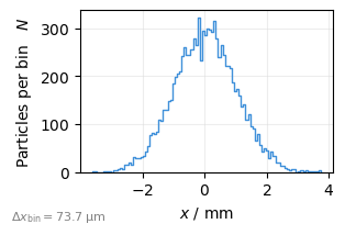
../_images/a1f9db1da2161b23460b73f9ec82a73249ee1551902644b4a35b79ea9511cae9.png

The only mandatory parameter is the property to be plotted ("x"). Most plots also accept a kind= parameter to plot different properties on subplots or twin axes. The data provided must contain or be suited to derive the requested properties. See below for a detailed description of properties, units and labels.

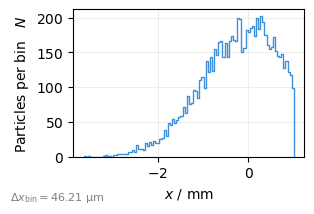
Most plots allso accept a mask= parameter to consider only a subset of the data:

plot = xplt.ParticleHistogramPlot("x", particles=data, mask=data.x < 1e-3)

../_images/21ad0a0955cd9fc61993bad579a3dc5ced6754cb187c7b6a606cae01ace77f77.png

Updating plot data#

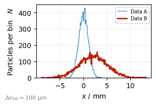
Plots can also be created blank, and the data updated later. This is very useful to create animations (see Animations):

plot = xplt.ParticleHistogramPlot(
    "x", bin_width=1e-4, plot_kwargs=dict(label="Data A")
)
plot.update(data);

../_images/2e6c53615a7e1e136294206772211ad7694bbe278ef08382af80abb319529d46.png

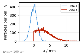
The parameter plot_kwargs= always allows to customize the artist. You can add more datasets:

plot.add_dataset(
    "ref",  # optional ID to update data later
    particles=data2,
    plot_kwargs=dict(label="Data B", c="C2", lw=2),
    autoscale=True,
)
plot.fig

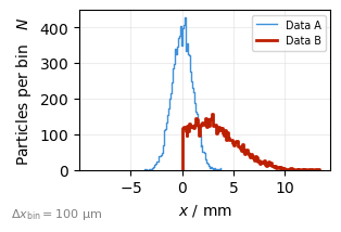
../_images/9e57f65f5e586d5f594a2c6aa0573a5892d7aa08a2741bb299e730566756d16a.png

…and update them as needed:

plot.update(data2, mask=data2.x > 0, dataset_id="ref")
plot.fig

../_images/5f848f9850160fc31587470e06fc5ef0c3df9e875e1df04a95e54324b17cac24.png

Tip

To add multiple datasets in a loop, pass add_default_dataset=False to the constructor to avoid the default artists from being created for you.

The parameter autoscale= of the xplt.ParticleHistogramPlot.add_dataset() and xplt.ParticleHistogramPlot.update() methods allows to specify the autoscale behaviour. By default, autoscaling is only performed on the first time data is supplied to the plot.
You can also manually autoscale the plot anytime:

plot.autoscale(axis="x", tight=False, reset=True)
plot.fig

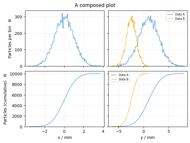
../_images/204c025a13d4212a630cbc8e77f4a891419ff3f6bc9769927b453afc62e79c2c.png

Composing plots#

By passing an existing axis to the constructor, it is possible to create composed plots (the axis shape must match the one otherwise created by the plot):

xplt.mpl.rcParams["figure.figsize"] = (6.4, 4.8)

fig, axs = plt.subplots(2, 2, sharex="col", sharey="row")
fig.suptitle("A composed plot")

for i, p in enumerate("xy"):
    for j, dat in enumerate((data, data2)):
        plot = xplt.ParticleHistogramPlot(
            p,
            dat,
            "count,cumulative",
            ax=axs[:, i],
            plot_kwargs=dict(label=dat.label, ls=f"-{j}"),  # customization
        )
        if i == 0:
            break

for a in axs[:, 1]:
    a.set(ylabel=None)

../_images/4128dd39eeab985945189f8142495da718ba95d14daccf183d61405324095137.png

Properties, Units and Labels#

Properties are what makes this library easy to use while still very flexible.

A property is anything that we can “get” from a dataset, either as an attribute data.xyz, an index data["xyz"] or even a column in a pandas dataframe.
For brevity, consider the following arbitrary dataset in the following:

# custom data
N = 10000
data = {
    "h": np.linspace(0, 100, num=N),
    "w": np.random.normal(size=N),
    "x": np.random.normal(size=N),
    "y": np.random.normal(size=N),
}

Now we can plot the x-y-phasespace simply by specifying exactly that:

plot = xplt.PhaseSpacePlot(data, "x-y", display_units=dict(y="m"))

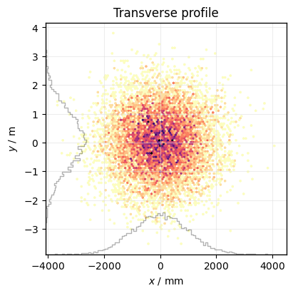
../_images/4bb7e704d53f83105759bbe96c02f4a748c9c84e0a20662231c8d4636eb55e61.png

This works, because both x and y are standard properties which are defined in the library with default settings for units, labels and symbols. Here specifically, the assumption is that x is provided in meters since that is the SI unit used by Xsuite, and that the default display unit for x should be millimeters. You can specify a display unit, and the data is automatically converted accordingly.

See below for a list of predefined properties and the default assumed. You can add or change properties and their respective units, labels and symbols if required. Futher, derived properties can easily be defined building on the already existing ones.

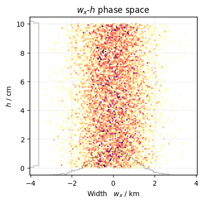
Adding custom data properties#

To define or overwrite properties of a data object with a certain unit or meaning, you can either register them globally:

# our data["w"] is the width in km
xplt.register_data_property("w", data_unit="km", symbol="$w_x$", description="Width")

Or on-the-fly for a single plot with the data_units parameter. Both enable automatic axes and legend labeling, as well as the use of the display_units parameter:

# our data["h"] is in mm, but we want to convert it to cm
plot = xplt.PhaseSpacePlot(
    data, "w-h", data_units={"h": "mm"}, display_units={"h": "cm"}
)

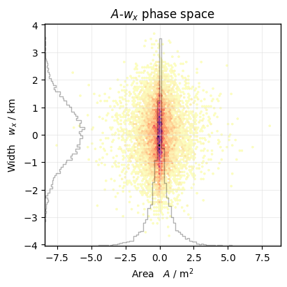
../_images/e5c913dd56d0050af565ab3eed89afa5ea3e92759c437985af41199dda12915d.png

Derived properties#

It is often useful to add properties that depend on already existing ones, e.g. if you simply want to plot the squareroot of a parameter, or have a complex expression. The function parameters must be valid property names, such that the data and units can be inferred automatically. It is also possible to specify the unit explicitly where necessary.

# since both x and y are know properties (in meter), A is known to be in square meter
xplt.register_derived_property("A", lambda x, y: x * y, description="Area")
# since the unit of `6` can not be inferred, we declare B to be in square meter too
xplt.register_derived_property("B", lambda A: A + 6, unit="m^2")

plot = xplt.PhaseSpacePlot(data, "A-w")

../_images/c75be35b27d8a4d4df1ecc8f507c712c2f92dc12ff31844b25051b331ba1f669.png

Default properties#

Global default properties applicable to all plots:

Property	Unit	Symbol	Description	Derived from
`at_turn`	\( \)	\(n\)	Turn
`charge_ratio`	\( \)	\(q/q_\mathrm{ref}\)	Charge ratio
`chi`	\( \)	\((q/q_\mathrm{ref})/(m/m_\mathrm{ref})\)	Charge-over-rest-mass ratio
`count`	\( \)	\(N\)	Count
`delta`	\( \)	\(\delta\)
`energy`	\( \mathrm{eV} \)	\(E\)	Total energy
`m`	\( \frac{\mathrm{eV}}{\mathrm{c}^{2}} \)	\(m\)	Rest mass	`chi` `charge_ratio` `mass0`
`mass0`	\( \frac{\mathrm{eV}}{\mathrm{c}^{2}} \)	\(m_\mathrm{ref}\)	Reference rest mass
`ptau`	\( \)	\(p_\tau\)
`px`	\( \)	\(x'\)
`py`	\( \)	\(y'\)
`pzeta`	\( \)	\(p_\zeta\)
`q`	\( \mathrm{e} \)	\(q\)	Charge	`q0` `charge_ratio`
`q0`	\( \mathrm{e} \)	\(q_\mathrm{ref}\)	Reference charge
`s`	\( \mathrm{m} \)	\(s\)
`tau`	\( \mathrm{m} \)	\(\tau\)
`x`	\( \mathrm{m} \)	\(x\)
`x_mean`	\( \mathrm{m} \)	\(\langle x \rangle\)
`x_std`	\( \mathrm{m} \)	\(\sigma_x\)
`y`	\( \mathrm{m} \)	\(y\)
`y_mean`	\( \mathrm{m} \)	\(\langle y \rangle\)
`y_std`	\( \mathrm{m} \)	\(\sigma_y\)
`zeta`	\( \mathrm{m} \)	\(\zeta\)

Particle plots#

These plots support normalized coordinates and action-angle-variables.

See Phasespace for usage examples

Additional default properties applicable only to: ParticleHistogramPlot ParticlesPlot PhaseSpacePlot SpillQualityPlot SpillQualityTimescalePlot TimeBinPlot TimeFFTPlot TimeIntervalPlot TimePlot

Property	Unit	Symbol	Derived from
`Jx`	\( \mathrm{m} \)	\(J_x\)	`X` `Px`
`Jy`	\( \mathrm{m} \)	\(J_y\)	`Y` `Py`
`Px`	\( \mathrm{m}^{0.5} \)	\(X'\)	`x` `px` `delta`
`Py`	\( \mathrm{m}^{0.5} \)	\(Y'\)	`y` `py` `delta`
`X`	\( \mathrm{m}^{0.5} \)	\(X\)	`x` `px` `delta`
`Y`	\( \mathrm{m}^{0.5} \)	\(Y\)	`y` `py` `delta`
`t`	\( \mathrm{s} \)	\(t\)	`_data` `at_turn` `zeta`
`zeta_wrapped`	\( \mathrm{m} \)	\(\zeta\)	`zeta`
`Θx`	\( \mathrm{rad} \)	\(Θ_x\)	`X` `Px`
`Θy`	\( \mathrm{rad} \)	\(Θ_y\)	`Y` `Py`

Histogram plots#

Additional default properties applicable only to: ParticleHistogramPlot TimeBinPlot TimeFFTPlot TimeIntervalPlot

Property	Unit	Symbol	Description
`charge`	\( \mathrm{e} \)	\(Q\)	Charge per bin
`count`	\( \)	\(N\)	Particles per bin
`cumulative`	\( \)	\(N\)	Particles (cumulative)
`current`	\( \frac{\mathrm{e}}{\mathrm{s}} \)	\(I\)	Current
`rate`	\( \frac{1}{\mathrm{s}} \)	\(\dot{N}\)	Particle rate

Spill quality plots#

Additional default properties applicable only to: SpillQualityPlot SpillQualityTimescalePlot

Property	Unit	Symbol	Description
`cv`	\( \)	\(c_\mathrm{v}=\sigma/\mu\)	Coefficient of variation
`duty`	\( \)	\(F=\langle N \rangle^2/\langle N^2 \rangle\)	Spill duty factor
`maxmean`	\( \)	\(M=\hat{N}/\langle N \rangle\)	Max-to-mean ratio

Floor plot#

See Beamline for usage examples

Additional default properties applicable only to: FloorPlot

Property	Unit	Symbol
`X`	\( \mathrm{m} \)	\(X\)
`Y`	\( \mathrm{m} \)	\(Y\)
`Z`	\( \mathrm{m} \)	\(Z\)
`phi`	\( \mathrm{rad} \)	\(\Phi\)
`psi`	\( \mathrm{rad} \)	\(\Psi\)
`theta`	\( \mathrm{rad} \)	\(\Theta\)

Twiss plot#

See Twiss for usage examples

Additional default properties applicable only to: TwissPlot

Property	Unit	Symbol	Derived from
`alfx`	\( \)	\(\alpha_x\)
`alfy`	\( \)	\(\alpha_y\)
`betx`	\( \mathrm{m} \)	\(\beta_x\)
`bety`	\( \mathrm{m} \)	\(\beta_y\)
`dpx`	\( \)	\(D_{x'}\)
`dpy`	\( \)	\(D_{y'}\)
`dx`	\( \mathrm{m} \)	\(D_x\)
`dy`	\( \mathrm{m} \)	\(D_y\)
`envelope3_x`	\( \mathrm{m} \)	\(x\pm3\sigma_x\)	`x` `sigma_x`
`envelope3_y`	\( \mathrm{m} \)	\(y\pm3\sigma_y\)	`y` `sigma_y`
`envelope_x`	\( \mathrm{m} \)	\(x\pm\sigma_x\)	`x` `sigma_x`
`envelope_y`	\( \mathrm{m} \)	\(y\pm\sigma_y\)	`y` `sigma_y`
`gamx`	\( \frac{1}{\mathrm{m}} \)	\(\gamma_x\)
`gamy`	\( \frac{1}{\mathrm{m}} \)	\(\gamma_y\)
`max_x`	\( \mathrm{m} \)	\(x_\mathrm{max}\)
`max_y`	\( \mathrm{m} \)	\(y_\mathrm{max}\)
`min_x`	\( \mathrm{m} \)	\(x_\mathrm{min}\)
`min_y`	\( \mathrm{m} \)	\(y_\mathrm{min}\)
`mux`	\( \)	\(\mu_x\)
`muy`	\( \)	\(\mu_y\)
`sigma_px`	\( \)	\(\sigma_{x'}\)
`sigma_py`	\( \)	\(\sigma_{y'}\)
`sigma_pzeta`	\( \)	\(\sigma_{p_\zeta}\)
`sigma_x`	\( \mathrm{m} \)	\(\sigma_x\)
`sigma_y`	\( \mathrm{m} \)	\(\sigma_y\)
`sigma_zeta`	\( \mathrm{m} \)	\(\sigma_\zeta\)