Twiss

This is an example of plotting lines and twiss results. First, create a simple line and a tracker:

Show imports Hide code cell content

%load_ext autoreload
%autoreload 2

import xtrack as xt
import xdeps as xd
import xpart as xp
import xplt
import numpy as np

xplt.apply_style()

Show line generation code Hide code cell content

## Generate a simple 6-fold symmetric FODO lattice

n = 6  # number of sections
elements = {
    "QF": xt.Multipole(length=0.3, knl=[0, +0.63]),
    "QD": xt.Multipole(length=0.3, knl=[0, -0.48]),
    "MU": xt.Multipole(length=0.5, knl=[np.pi / n], hxl=[np.pi / n]),
}
parts = {
    "a": [
        xt.Node(0.7, "QF"),
        xt.Node(1.4, "MU"),
        xt.Node(2.1, "QD"),
        xt.Node(2.8, "MU"),
    ],
    "b": [
        xt.Node(2.2, "MU"),
        xt.Node(2.9, "QD"),
        xt.Node(3.6, "MU"),
        xt.Node(4.3, "QF"),
    ],
}
nodes = [xt.Node(5.0 * i, "a" if i % 2 else "b", name=f"S{i+1}") for i in range(n)]

# sextupoles
for i in range(n):
    sx = xt.Multipole(length=0.2, knl=[0, 0, 0.5 * np.sin(2 * np.pi * (i / n))])
    nodes.append(xt.Node(0.2, sx, from_=f"S{i+1}", name=f"S{i+1}SX"))

# apertures
nodes.append(xt.Node(5, xt.LimitRect(min_x=-5e-3, max_x=3e-3, max_y=3e-3)))
nodes.append(xt.Node(10, xt.LimitRectEllipse(max_x=6e-3, max_y=1)))

line = xt.Line.from_sequence(
    nodes, length=5.0 * n, sequences=parts, elements=elements, auto_reorder=True
)
line.particle_ref = xp.Particles()
line.build_tracker();

Then determine it’s twiss parameters. Use the at_s parameter to get the twiss data with high resolution as a function of s (rather than at each element only).

tw = line.twiss(
    method="4d", at_s=np.linspace(0, line.get_length(), 500, endpoint=False)
)

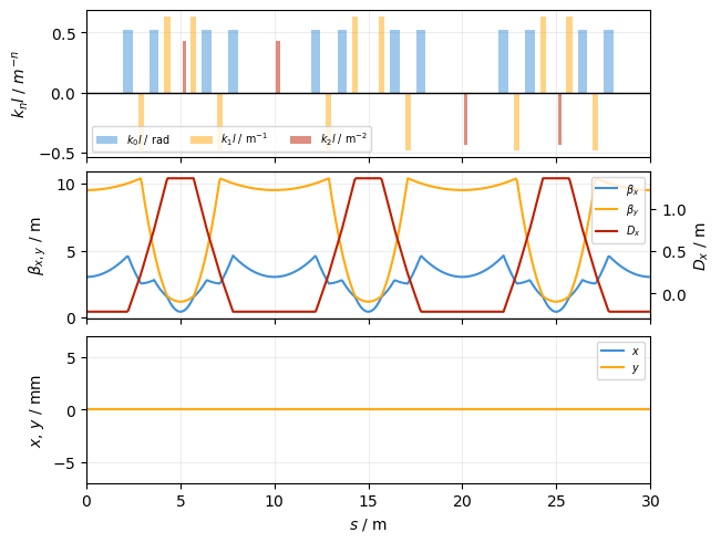
Default twiss plot

Create a default TwissPlot (passing line to the plot adds a beamline plot to the top):

plot = xplt.TwissPlot(tw, line=line)
plot.axis("x").set(ylim=(-7, 7));

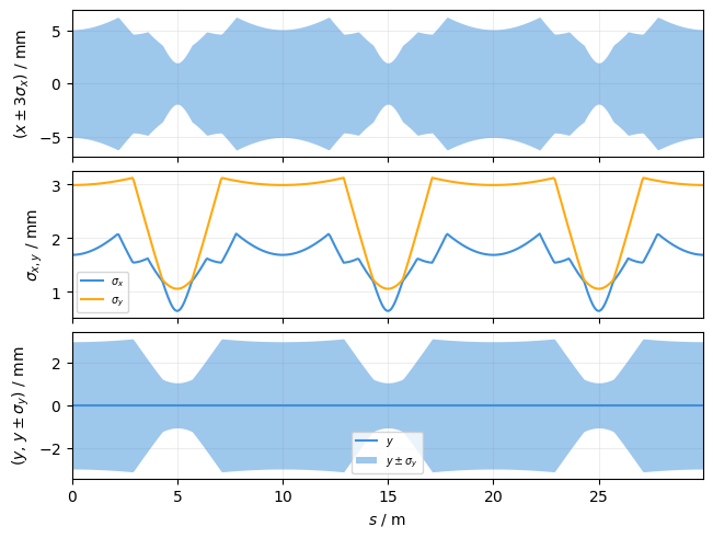
Beam size plot

You can also plot the beam size and envelope:

# Normalized emittance in m*rad
cv = tw.get_betatron_sigmas(nemitt_x=1e-6, nemitt_y=1e-6)

plot = xplt.TwissPlot((tw, cv), "envelope3_x, sigma, y + envelope_y")

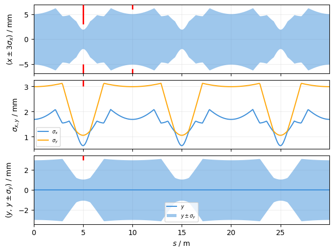
Apertures

You can also plot apertures onto the existing plot:

ap = xplt.util.apertures(line)
xd.Table(ap, index="s").to_pandas()

	s	min_x	max_x	min_y	max_y
0	5.0	-0.005	0.003	-1.000000e+10	0.003
1	10.0	-0.006	0.006	-1.000000e+00	1.000

plot.plot_apertures(ap, lw=2, color="r")
plot.fig

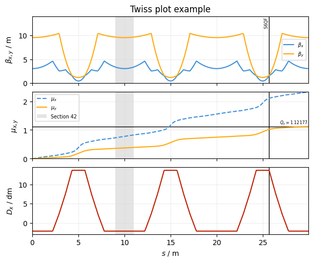
Customisation

Use the parameter kind to specify what is plotted. This is a string specifying the properties to be plotted, separated by , for each subplot. Use a+b to plot multiple properties on an axis and a-b to separate left and right axis. See TwissPlot for details.

A list with all supported properties can be found in Common concepts under Default properties and Twiss plot.

Tip

Use prefix notation as shorthand to plot both x- and y-properties, e.g. bet for betx+bety

plot = xplt.TwissPlot(
    tw,
    kind="bet,mux+muy,dx",  # 3 subplots: plot beta functions ("bet"="betx+bety") on the first,
    #                                     phase advances on the second, and dispersion on the third
    display_units=dict(d="dm"),  # dispersion in deci-meter ("d=" for "dx" and "dy")
    figsize=(6, 5),
)

# add some annotations
plot.axline("s", line.get_s_position("S6QF"), annotation="S6QF")
plot.axspan("s", 9, 11, label="Section 42")
plot.axline("muy", tw.qy, annotation=f"$Q_y={tw.qy:g}$", annotation_loc=1)

# adjust some axes
plot.axis(0).set(title="Twiss plot example", ylim=(0, 14))
plot.axis("mux").set(ylim=(0, tw.qx))

# adjust line layout
plot.artist("mux").set(ls="--")
plot.artist(subplot=2).set(c="pet2")

# legend is shown by default for subplots with more than 1 trace
plot.legend(1, loc="upper left")  # call it manually to reflect updated line layout
# plot.legend() # uncomment this to show legends on all subplots

---

See also

• xplt.twiss