Hamiltonians

This is an example of plotting hamiltonians in phase space distributions. First, create a simple line, a tracker and a particle set:

Show imports Hide code cell content

%load_ext autoreload
%autoreload 2

import xtrack as xt
import xpart as xp
import xplt
import numpy as np

xplt.apply_style()

np.random.seed(43543557)

Show line generation code Hide code cell content

## Generate a simple 6-fold symmetric FODO lattice

n = 6  # number of sections
elements = {
    "QF": xt.Multipole(length=0.3, knl=[0, +0.63]),
    "QD": xt.Multipole(length=0.3, knl=[0, -0.48]),
    "MU": xt.Multipole(length=0.5, knl=[np.pi / n], hxl=[np.pi / n]),
}
parts = {
    "a": [
        xt.Node(0.7, "QF"),
        xt.Node(1.4, "MU"),
        xt.Node(2.1, "QD"),
        xt.Node(2.8, "MU"),
    ],
    "b": [
        xt.Node(2.2, "MU"),
        xt.Node(2.9, "QD"),
        xt.Node(3.6, "MU"),
        xt.Node(4.3, "QF"),
    ],
}
nodes = [xt.Node(5.0 * i, "a" if i % 2 else "b", name=f"S{i+1}") for i in range(n)]

# sextupoles
for i in range(n):
    sx = xt.Multipole(length=0.2, knl=[0, 0, 0.5 * np.sin(2 * np.pi * (i / n))])
    nodes.append(xt.Node(0.2, sx, from_=f"S{i+1}", name=f"S{i+1}SX"))

# aperture
nodes.append(xt.Node(0, xt.LimitRect(min_x=-0.01, max_x=0.01), name="APERTURE"))

line = xt.Line.from_sequence(
    nodes, length=5.0 * n, sequences=parts, elements=elements, auto_reorder=True
)
line.particle_ref = xp.Particles()
line.build_tracker();

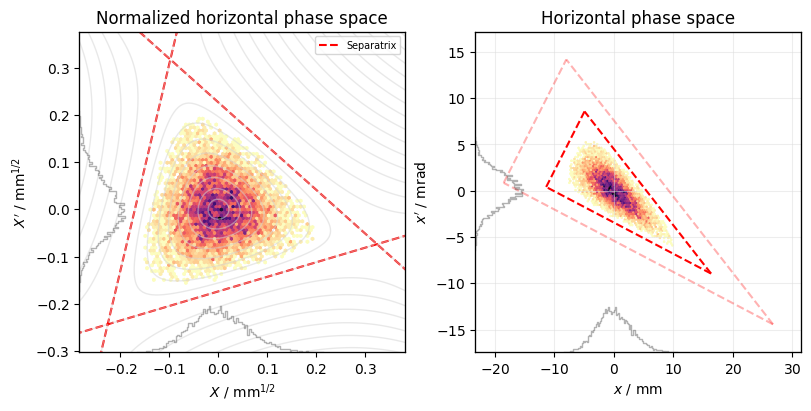
Kobayashi Hamiltonian

The Kobayashi Hamiltonian describes the particle dynamics in the vicinity of a driven 3rd order resonance:

\[\begin{equation*} H = 3\pi d \left(X^2 + X'^2\right) + \frac{S}{4} \left(3 X X'^2 - X^3\right) \end{equation*}\]

with the tune distance d=q-r to the third integer resonance r=n/3 and the normalized sextupole strength:

\[\begin{equation*} S = -\frac{1}{2} \beta_x^{3/2} k_2 l \end{equation*}\]

Show particle generation code Hide code cell content

## Generate particles
nparticles = int(1e4)

# Transverse distribution (gaussian)
norm_emitt_x = 4e-6  # normalized 1-sigma emittance in m*rad (=beta*gamma*emitt_x)
norm_emitt_y = 1e-6  # normalized 1-sigma emittance in m*rad (=beta*gamma*emitt_y)
x, px = xp.generate_2D_gaussian(nparticles)
y, py = xp.generate_2D_gaussian(nparticles)

# Longitudinal distribution (coasting beam)
rel_momentum_spread = 1e-4  # relative momentum spread ( P/p0 - 1 )
zeta = line.get_length() * np.random.uniform(-0.5, 0.5, nparticles)
delta = rel_momentum_spread * xp.generate_2D_gaussian(nparticles)[0]

particles = line.build_particles(
    x_norm=x,
    px_norm=px,
    nemitt_x=norm_emitt_x,
    y_norm=y,
    py_norm=py,
    nemitt_y=norm_emitt_y,
    method="4d",  # for twiss (default is 6d, won't work without a cavity)
    zeta=zeta,
    delta=delta,
)

Show tracking code Hide code cell content

## Track for a few turns and then stop at the sextupole
line.track(particles, num_turns=500, ele_stop=7)
print(f"{np.sum(particles.state <= 0)} of {len(particles.state)} particles lost")

## Determine twiss parameters for normalized phase space plots
tw = line.twiss(method="4d", at_elements=[7])

print(f"qx: {tw.qx:g}")

549 of 10000 particles lost
qx: 2.33247

Phase space plot with separatrix and equipotential lines:

plot = xplt.PhaseSpacePlot(
    particles,
    mask=particles.state > 0,
    kind="X,x",
    # plot='scatter',
    twiss=tw,
    hist_kwargs=dict(gridsize=50),
)

# determine the virtual sextupole
S, mu = xplt.util.virtual_sextupole(line, verbose=True)

# plot the hamiltonian
plot.plot_hamiltonian_kobayashi(0, S=S, mu=mu, extend=5)
plot.plot_hamiltonian_kobayashi(1, S=S, mu=mu, equipotentials=False)
plot.plot_hamiltonian_kobayashi(
    1,
    S=S,
    mu=mu,
    equipotentials=False,
    delta=3e-4,
    separatrix_kwargs=dict(alpha=0.3),
)
plot.axis(0).legend();

Sextupoles
  name       k2l     betx      mux        dx    S_abs       S_deg
  S2SX   0.43301  0.53530  0.45590   1.36368  0.08479   -47.62808
  S3SX   0.43301  3.05592  0.78793  -0.21368  1.15660   -49.03026
  S4SX   0.00000  0.53530  1.23339   1.36368  0.00000    72.05980
  S5SX  -0.43301  3.05592  1.56542  -0.21368  1.15660  -109.34238
  S6SX  -0.43301  0.53530  2.01088   1.36368  0.08479    11.74769
  ---------------------------------------------------------------
  Virtual sextupole: S = 2.07503 m^(-1/2) at mu = -0.0700163 rad/2pi

---

See also

• xplt.phasespace